v0.10 — model and validation details
This record is for readers reviewing implementation choices and numerical evidence. Start with Demo and Method for an introduction. Figures use public TT04 or synthetic data; they are model results, not measured wafers.
Contents
- 1. Changes and candidate priority
- 2. Presets and reference pattern
- 3. Relative dose and threshold
- 4. Source, pixel and cost comparisons
- 5. Bounded ambit validation
- 6. 0.1 nm DBU and contours
- 7. Large-contour processing cost
- 8. Focus–dose / Process Window
- 9. Interpretation and regression checks
- 10. Data downloads
1. Candidate priority: smaller CD, then larger area
Both width and space use ascending measured_dbu, descending area_dbu2, then the existing deterministic bounding-box tie breaker. Missing CD ranks last. Area means the merged DRC candidate marker, not the original conductor polygon.
| Comparison | First candidate |
|---|---|
| Width: CD 80 / large area vs CD 90 / small area | CD 80 |
| Space: CD 80 / small area vs CD 90 / large area | CD 80 |
| Equal CD, different area | Larger area for both width and space |
| Missing measured CD | After measured candidates |
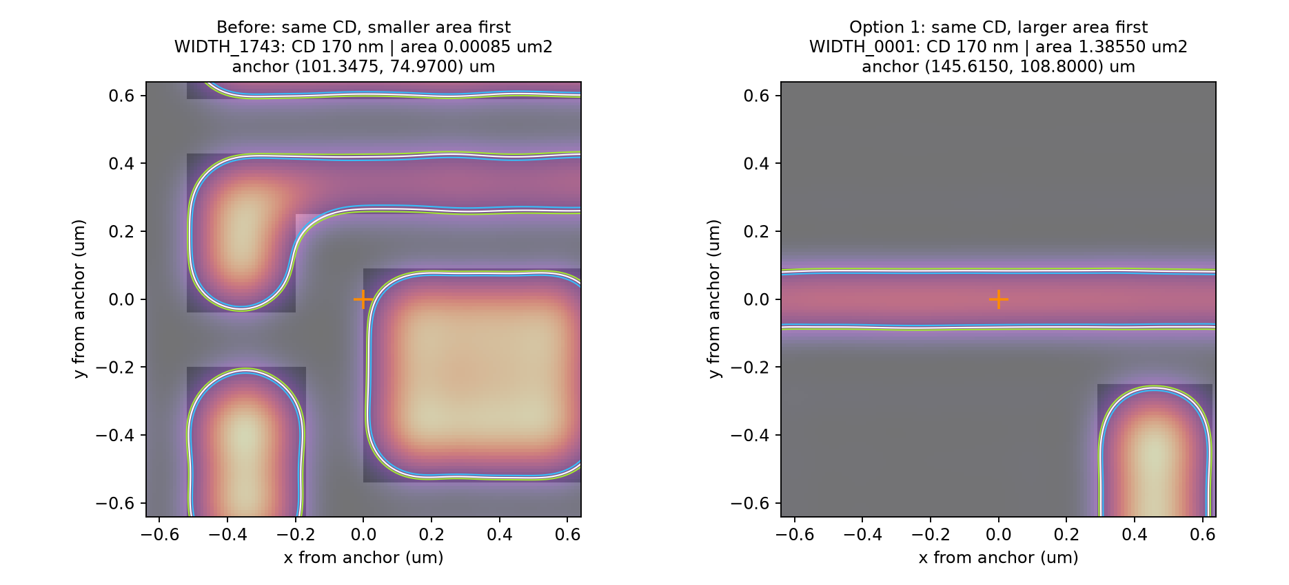
The previous smaller-area tie breaker selected a 170 nm width interaction with only 5 nm parallel overlap at a corner. Larger-area priority selects a long line at (145.615, 108.800) um: geometry CD 170 nm, marker area 1.38550 um². All 1,929 raw width components remain available. The experimental blanket short-overlap exclusion was not adopted.
The original minimum-distance edge-pair anchor convention remains. Area ordering is not a line-end detector: it can select the center of a long straight line. Component ordering and anchor selection are separate; candidate IDs can change with ordering. The separate calibration reference is excluded from minimum-CD hotspot summaries.
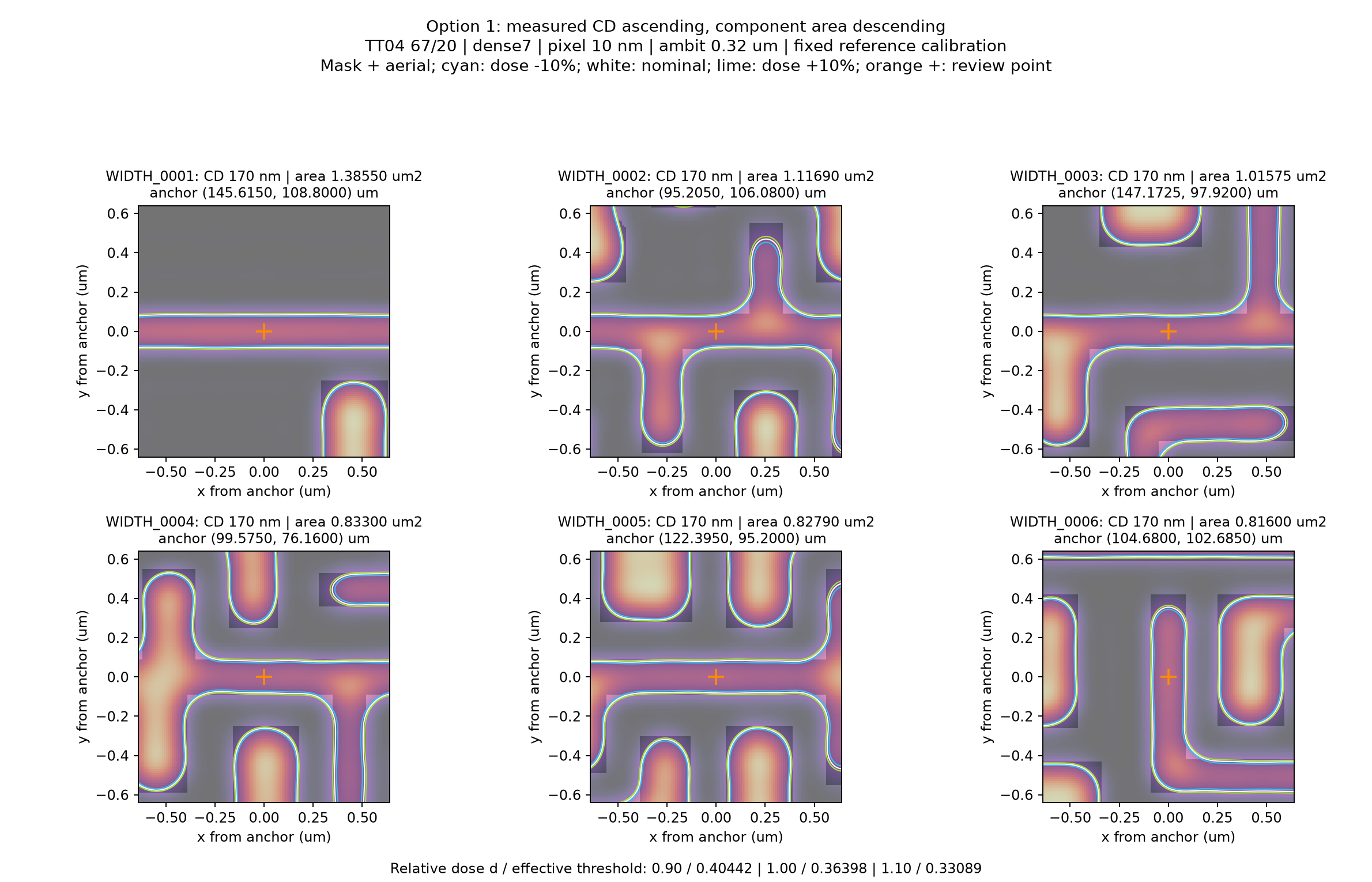
Each panel shows a 1.28 um crop around its anchor. Marker area also includes parts outside the crop. Orange crosses mark anchors. The warm-colored aerial image overlays the mask; cyan, white and lime outlines show relative dose −10% / nominal / +10%. Background color scaling is for display; quantitative contours use raw intensity.
Six leading space candidates
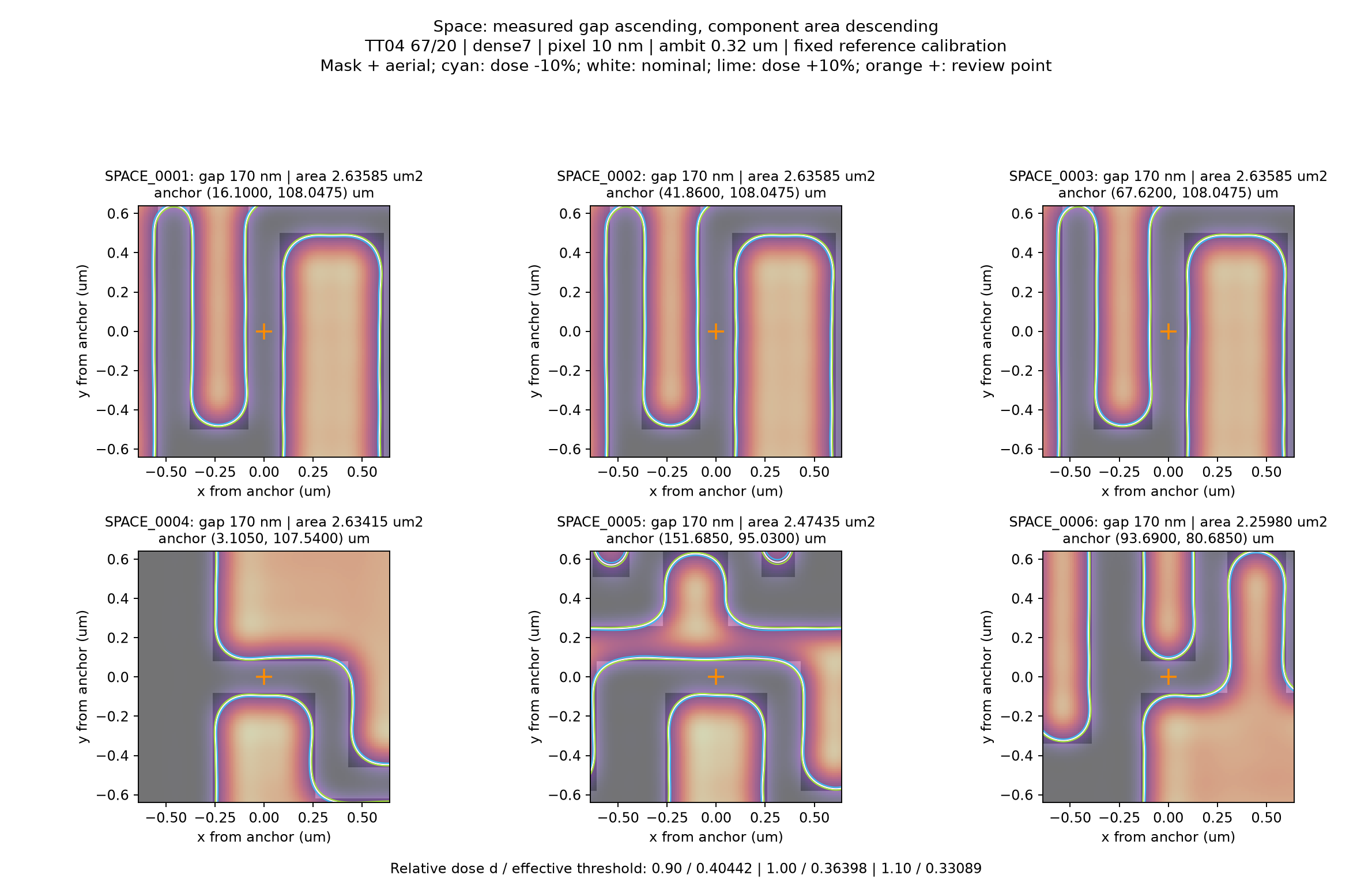
The six leading space candidates use the same ordering, Speed optics and fixed reference calibration. The first three are repeated patterns at different coordinates, not duplicate images. Panel gap values describe the input geometry.
2. Presets and reference pattern
| Setting | Speed / demo | Internal / evaluation |
|---|---|---|
| Source | dense7: 29 points | dense11: 81 points |
| Wavelength / NA / sigma | 248 nm / 0.68 / 0.60 | Same |
| Pixel / inner ROI | 10 nm / 2.56 um | Same |
| Ambit / raster | 0.32 um / 320 x 320 | Same |
| Geometry DBU | 0.1 nm | 0.1 nm |
| Filled contours | d = 0.9 / 1.0 / 1.1 | d = 0.9 / 1.0 / 1.1 |
| Detailed Region screening | Off; opt-in nominal dose | All three preview doses |
Illumination is conventional circular. Dense11 is the balanced internal-evaluation choice; dense7 is the faster Render-demo choice. They are not interchangeable numerical results. Dense grid labels differ from the actual number of points inside the circular source.
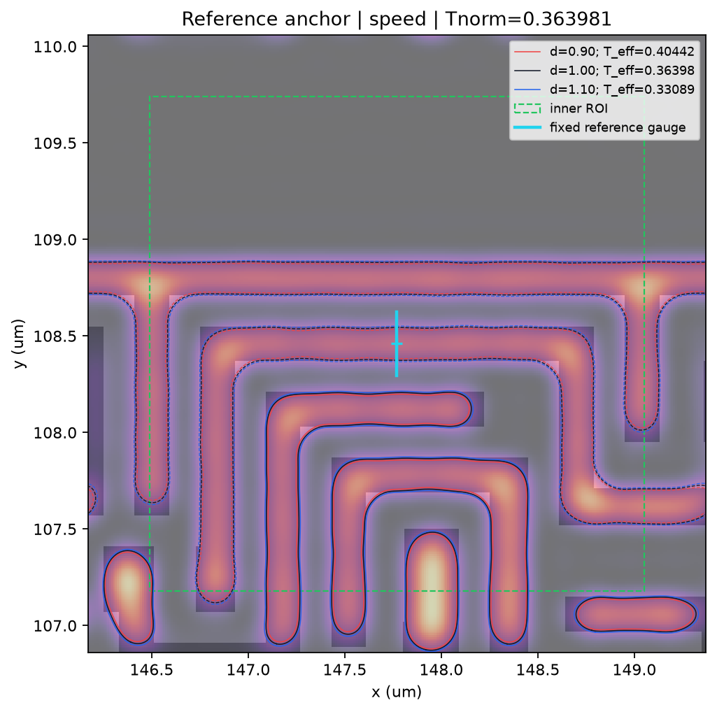
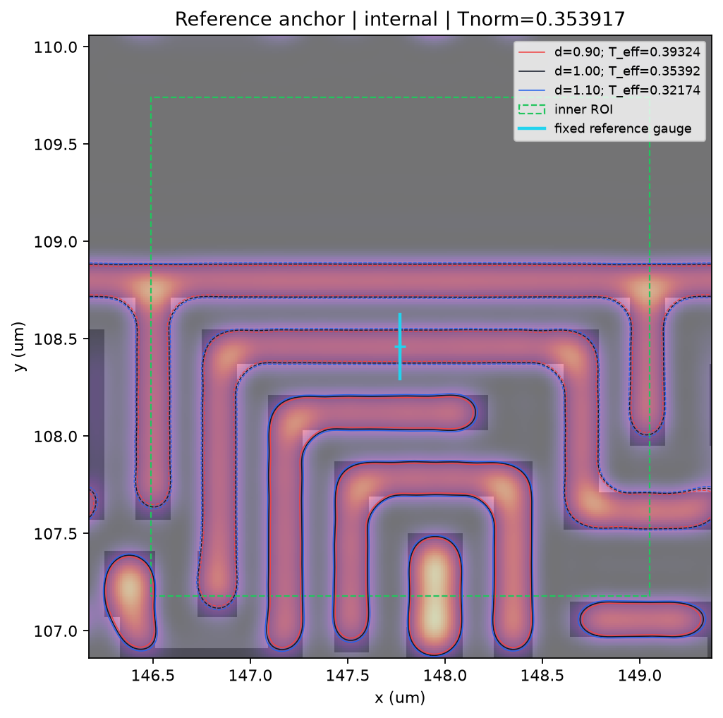
The reference is a dense 170 nm line and adjacent gaps on TT04 PWM layer 67/20 at (147.770, 108.460) um. Registered references require matching input hash and layer. Other inputs require a gauge location, direction and design CD verified against geometry. This validation snapshot uses two ranked candidates plus one reference; the web default uses five ranked candidates.
3. Relative dose, T0, D0 and Tnorm
The model is D0 × d × I(x,y,z) >= T0. On the per-unit-dose image, this is I >= T_eff = T0 / (D0 × d) = Tnorm / d.
| Symbol | Meaning |
|---|---|
| I | Raw clear-field-relative aerial intensity per unit dose |
| T0 | Fixed model resist threshold, 0.30 here |
| D0 | Nominal dose-to-size scale fitted to the design reference CD |
| d | Relative dose compared with D0: 0.90 / 1.00 / 1.10 |
| Tnorm | T0 / D0, fitted nominal image threshold |
| T_eff | Tnorm / d, effective image threshold for each relative dose |
Changing dose does not change T0 itself. Higher dose corresponds to lower T_eff. A ±10% dose change is not a ±0.1 threshold change. The fitted ratio T0/D0 determines these results; its terms are not independently identified material properties. No physical mJ/cm² exposure claim is made.
The existing PW FocusDoseSweepConfig, effective_threshold() and dose-to-size calibration are reused. Best-focus coarse search is followed by bracket refinement as needed. Refinement updates thresholds and fixed-gauge crossings without recalculating the optical image. Nominal fitting tolerance is 0.1 nm. Failed or out-of-tolerance calibration makes quantitative results unavailable; it does not trigger an arbitrary-threshold fallback.
Dose contours, CD/space and PW use raw clear-field-relative intensity. Per-ROI peak or min/max normalization would erase relevant focus-dependent peak/contrast changes and invalidate the dose convention. Display normalization is separate. Historical 0.2 / 0.3 / 0.4 threshold figures are legacy visualization, not current dose conditions.
| Preset | Relative dose d | T0 | D0 | T_eff | Reference CD (nm) |
|---|---|---|---|---|---|
| speed | 0.90 | 0.30 | 0.82421875 | 0.404423 | 152.019 |
| speed | 1.00 | 0.30 | 0.82421875 | 0.363981 | 170.018 |
| speed | 1.10 | 0.30 | 0.82421875 | 0.330892 | 184.658 |
| internal | 0.90 | 0.30 | 0.84765625 | 0.393241 | 152.296 |
| internal | 1.00 | 0.30 | 0.84765625 | 0.353917 | 169.979 |
| internal | 1.10 | 0.30 | 0.84765625 | 0.321743 | 184.384 |
The 0.018 / 0.021 nm values are residuals of fitting the model to design CD, not printed-CD prediction accuracy or evidence of optical resolution finer than 10 nm pixels. Calibration depends on optics, numerical settings and reference geometry. Actual process-model calibration uses measured CDs from multiple patterns and focus–exposure data. Mack et al., Improved Methods for Lithography Model Calibration.
4. Source, pixel and cost: exploratory setting comparison
The table and two figures below precede raster-boundary stabilization. They are exploratory evidence, not current preset Tnorm values or final accuracy claims. They fix one anchor, 2.56 um ROI, focus 0/+0.2 um, dose 0.9/1/1.1, a central width and two neighboring spaces. Baseline Tnorm is frozen rather than refitted for every case. Dense31 / 5 nm / ambit 0.64 um is a finite numerical reference, not physical truth.
| Case | Source points | Pixel nm | Ambit um | Raster | Max CD delta vs ref (nm) | Max edge delta (nm) | Optics s | Runtime ratio | Traced peak MiB |
|---|---|---|---|---|---|---|---|---|---|
| baseline | 29 | 10 | 0.32 | 320 x 320 | 7.108 | 9.004 | 0.133 | 1.00 | 18.3 |
| source11 | 81 | 10 | 0.32 | 320 x 320 | 1.094 | 5.427 | 0.352 | 2.64 | 18.3 |
| source13 | 113 | 10 | 0.32 | 320 x 320 | 0.480 | 5.990 | 0.481 | 3.61 | 18.3 |
| pixel20 | 29 | 20 | 0.32 | 160 x 160 | 22.771 | 12.235 | 0.014 | 0.10 | 4.6 |
| pixel5 | 29 | 5 | 0.32 | 640 x 640 | 7.974 | 4.292 | 0.778 | 5.84 | 73.3 |
| ambit16 | 29 | 10 | 0.16 | 288 x 288 | 9.366 | 8.610 | 0.099 | 0.74 | 15.1 |
| ambit50 | 29 | 10 | 0.5 | 356 x 356 | 3.562 | 7.745 | 0.298 | 2.24 | 22.4 |
| ambit64 | 29 | 10 | 0.64 | 384 x 384 | 3.423 | 6.903 | 0.226 | 1.70 | 25.9 |
| joint13 | 113 | 5 | 0.64 | 768 x 768 | 0.816 | 0.919 | 3.811 | 28.63 | 103.5 |
| joint21 | 317 | 5 | 0.64 | 768 x 768 | 1.235 | 0.701 | 13.014 | 97.78 | 103.6 |
| joint31 | 709 | 5 | 0.64 | 768 x 768 | 0.000 | 0.000 | 28.561 | 214.59 | 103.7 |
| quality13 | 113 | 10 | 0.64 | 384 x 384 | 1.133 | 5.518 | 1.328 | 9.98 | 25.9 |
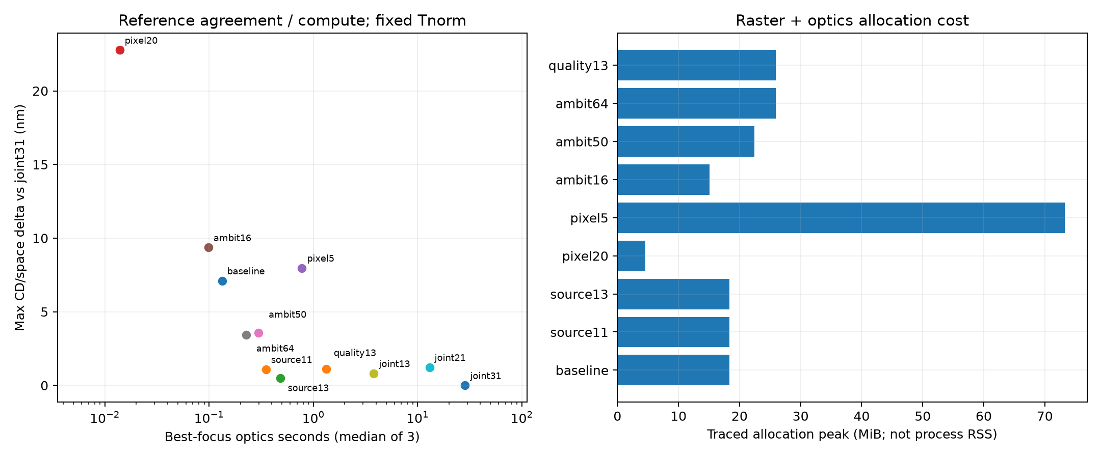
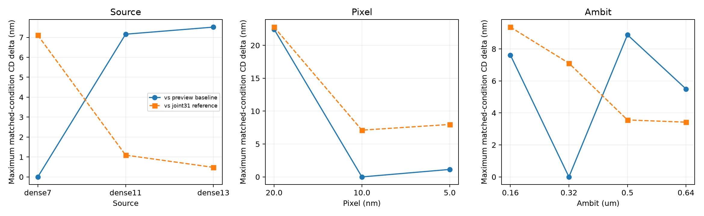
Best-focus optics uses the median of three runs under the same instrumentation. Traced peak means Python-tracked allocation, not total process peak or hosted memory. Source points × raster pixels is a workload proxy, not FLOPs. Changing pixel size also changes geometry rasterization; it must be distinguished from source sampling.
The 20 nm case is fast but differs substantially on this gauge; 5 nm raises computation cost. The operational compromise remains 10 nm. Dense11 is the first choice for balanced internal evaluation, dense7 the speed-oriented demo alternative. The earlier interpretation of dense13 component counts as central-pattern degradation was withdrawn after follow-up inspection. This table does not establish universally optimal sampling or convergence.
summary.csv · costs.csv · measurements.csv
5. Bounded ambit check with stabilized raster handling
These results were recomputed after raster-boundary stabilization. They fix the dense reference, gauges, 10 nm pixels, 2.56 um ROI and optics. Central width and neighboring spaces are compared at focus 0/+0.2 um and dose 0.9/1/1.1. Same-pixel comparisons reuse a master raster crop and verify identical inner coordinates and masks.
Dense7 and dense11 are independently fitted at 0.32 um. Dense11 ambit 0.32 / 0.50 / 0.64 uses frozen 0.32 Tnorm, so refitting cannot hide context differences. The table reports maximum absolute differences across those conditions. Edge differences are one-sided fixed-gauge crossings, not full-contour EPE.
| Comparison | Max CD/space difference (nm) | Max gauge-edge difference (nm) |
|---|---|---|
| dense7_32 vs dense11_32 | 6.495 | 3.660 |
| dense11_50 vs dense11_32 | 4.166 | 2.184 |
| dense11_64 vs dense11_32 | 2.812 | 1.937 |
| dense11_50 vs dense11_64 | 5.446 | 3.920 |
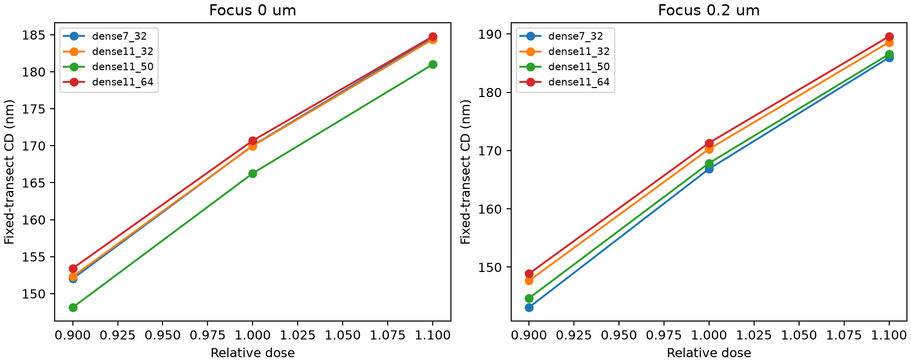
Differences do not decrease monotonically, and sub-1 nm convergence is not established. 0.32 um remains a cost-conscious study/demo choice. The 0.64 um case is only the largest context in this bounded comparison, not ground truth. Ambit also changes the FFT domain and frequency sampling.
Ambit is padding outside the inner ROI, not distance from the anchor. A centered anchor is 1.28 + 0.32 = 1.60 um from the outer boundary. 0.61 λ/NA ≈ 0.2225 um is the Airy first-zero radius scale. The approximately 1.44 ratio is retrospective, not a physical optimization criterion. At 10 nm pixels, 0.32 um gives 32 padding pixels and a 320 × 320 raster; that convenience is not a convergence guarantee.
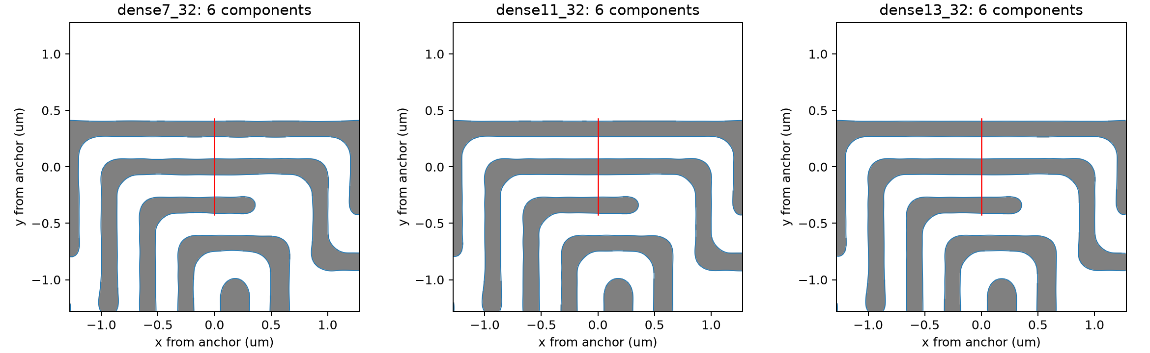
With stabilized boundary handling, inspected dense7/11/13 conditions each have six inner components and three central-strip components. Equal counts do not prove full topology equivalence. NILS values in the data remain fixed-transect proxies and are not used as a universal quality ranking.
measurements.csv · deltas.csv · costs.csv · local_connectivity.csv · calibration.json
6. 0.1 nm DBU and float contours to pya Regions
Input is rescaled to internal 0.1 nm DBU while preserving physical size and hierarchy. Optical intensity and contour extraction remain floating point; filled contour outer/hole associations are preserved when converting to pya Regions. DBU is a coordinate grid, distinct from 10 nm optical pixels or process accuracy. It does not create information absent from the input.
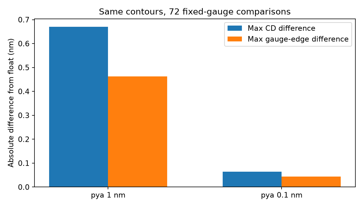
The following 72 fixed-gauge comparisons use identical contours represented as float, pya 1 nm and pya 0.1 nm.
| Representation | Max CD difference from float (nm) | Max gauge-edge difference (nm) |
|---|---|---|
| Float | 0 | 0 |
| pya 1 nm | 0.670 | 0.463 |
| pya 0.1 nm | 0.064 | 0.043 |
Open contours follow sampled-domain boundaries rather than arbitrary closing chords; holes and islands are preserved. Region width/space checks use the full sampled domain with Euclidean metrics, a 90° ignore angle and shielding. A rule-distance guard excludes artificial domain edges. Retained pairs are clipped to the inner ROI and marker polygons merged. This is separate from fixed-gauge CD.
Raster-boundary sensitivity exposed by DBU conversion was stabilized by snapping only numerical noise within 1e-8 pixel of integer pixel centers. Holes are applied per polygon before union, preserving other polygons’ islands. TT04 masks represented at 1 nm and 0.1 nm input DBU match. Pre-fix Tnorm values are not reused as current calibration.
measurements.csv · conversion.csv
7. Large-contour processing cost
| Grid (nm; 0=float) | Vertices | Geometry (s) | pya DRC (s) | Process peak (MiB) |
|---|---|---|---|---|
| 0 | 112153 | 0.262 | N/A | 91.4 |
| 0.1 | 112153 | 0.257 | 27.684 | 345.2 |
| 1 | 112153 | 0.235 | 11.948 | 217.0 |
| 0 | 28505 | 0.060 | N/A | 52.1 |
| 0.1 | 28505 | 0.095 | 5.673 | 122.6 |
| 1 | 28505 | 0.098 | 2.937 | 97.7 |
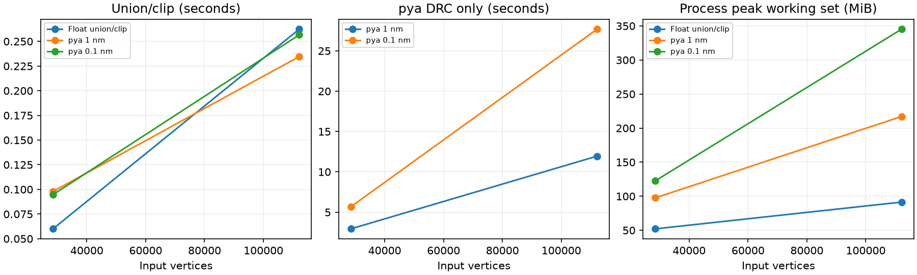
Identical contour rings feed float Shapely and pya union/clip. DRC is measured only for pya, so no float-versus-pya DRC speedup is claimed. The 0.1 nm grid retains more short edges and pairs and costs more than 1 nm. Values are single local runs in separate processes; peak working set is total process memory, not traced allocation or Render response time. Full-chip scaling still needs bounded tile/ROI execution and marker management.
8. Focus–dose / Process Window with the new ordering
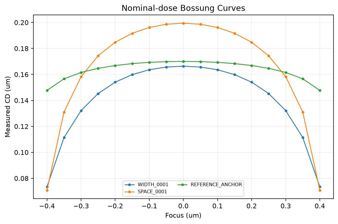
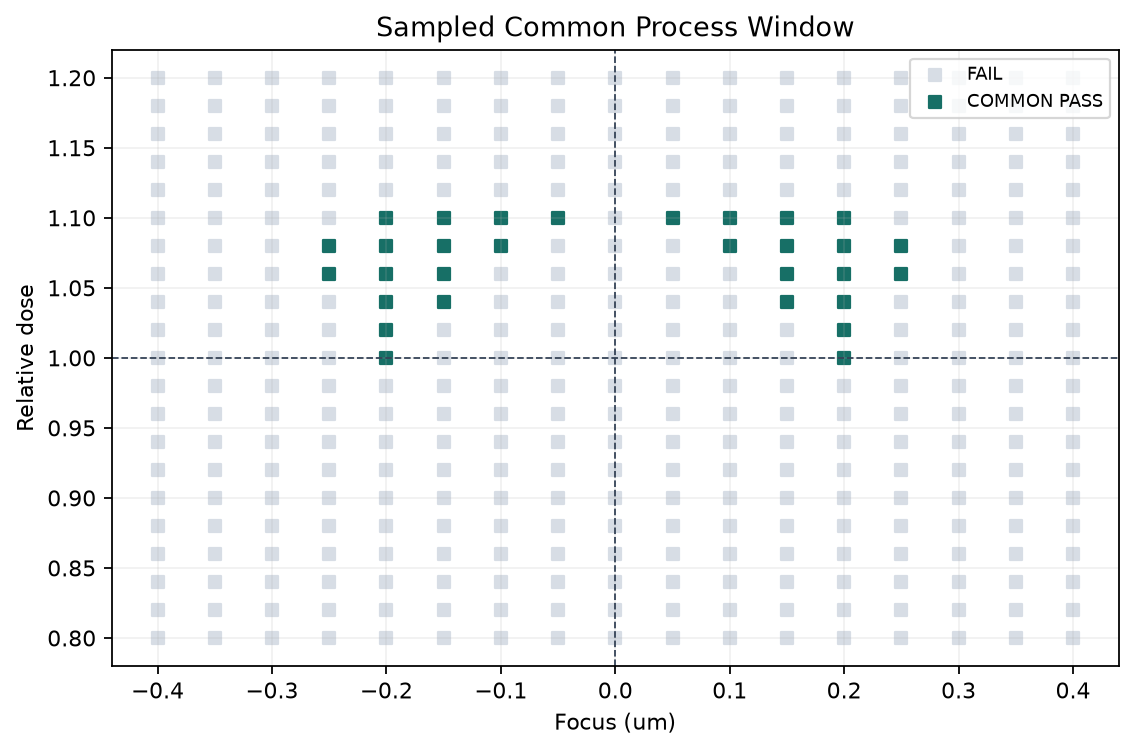
Both presets were rerun with the new ordering. Focus spans −0.40…+0.40 um in 0.05 um steps; relative dose spans 0.80…1.20 in 0.02 steps. There are 357 conditions × two candidates and one reference = 1,071 measurement rows. Nominal values below use the new width candidate and the existing space candidate at fixed gauges.
| Preset | Width candidate CD (nm) | Space candidate gap (nm) | Reference CD (nm) |
|---|---|---|---|
| speed | 166.340 | 199.443 | 170.018 |
| internal | 170.490 | 194.369 | 169.979 |
| Preset | Conditions / rows | Local wall time (s) | Process peak (MiB) | Reference fit residual (nm) |
|---|---|---|---|---|
| speed | 357 / 1,071 | 16.78 | 371.9 | 0.018074 |
| internal | 357 / 1,071 | 57.08 | 484.8 | 0.021365 |
The PW CD acceptance band is ±10% of each fixed gauge design target. DoF and exposure latitude summarize passing intervals on this discrete grid; continuous process limits between sampled conditions are not established.
speed
internal
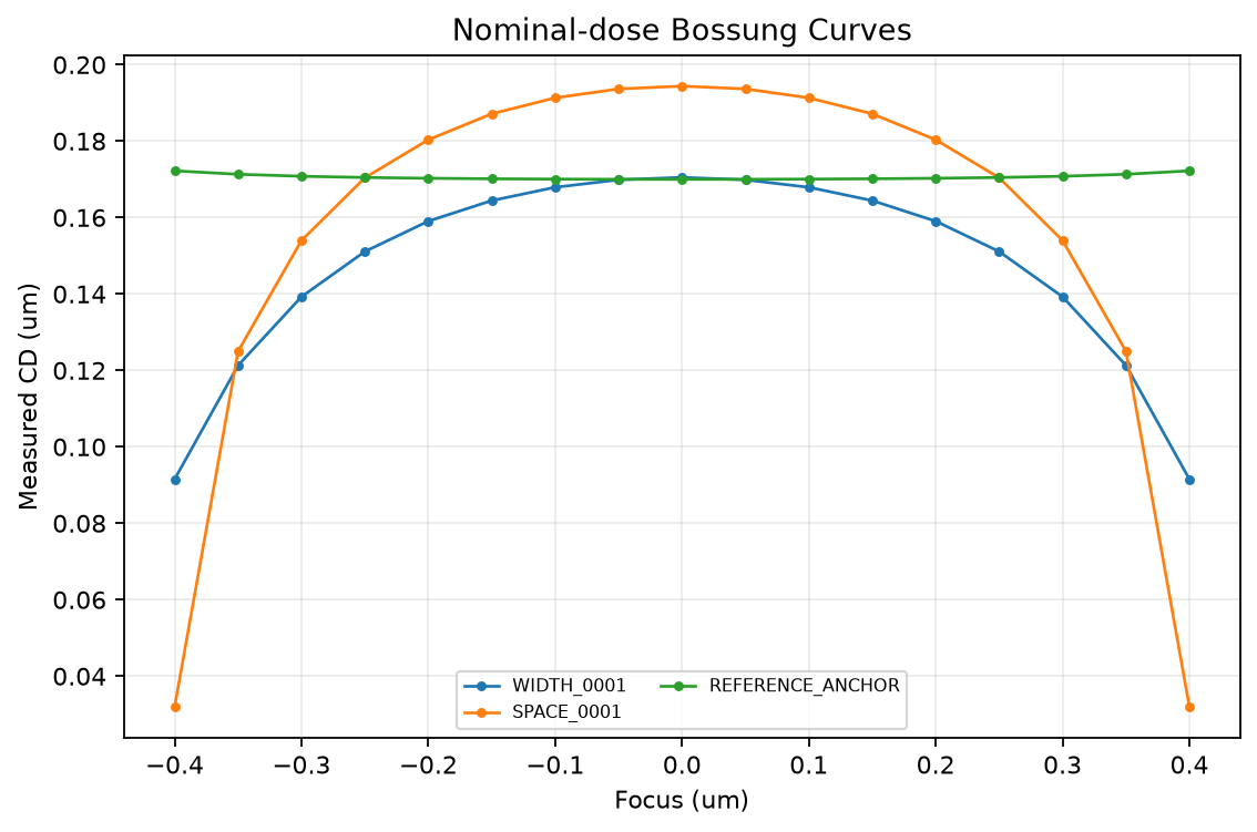
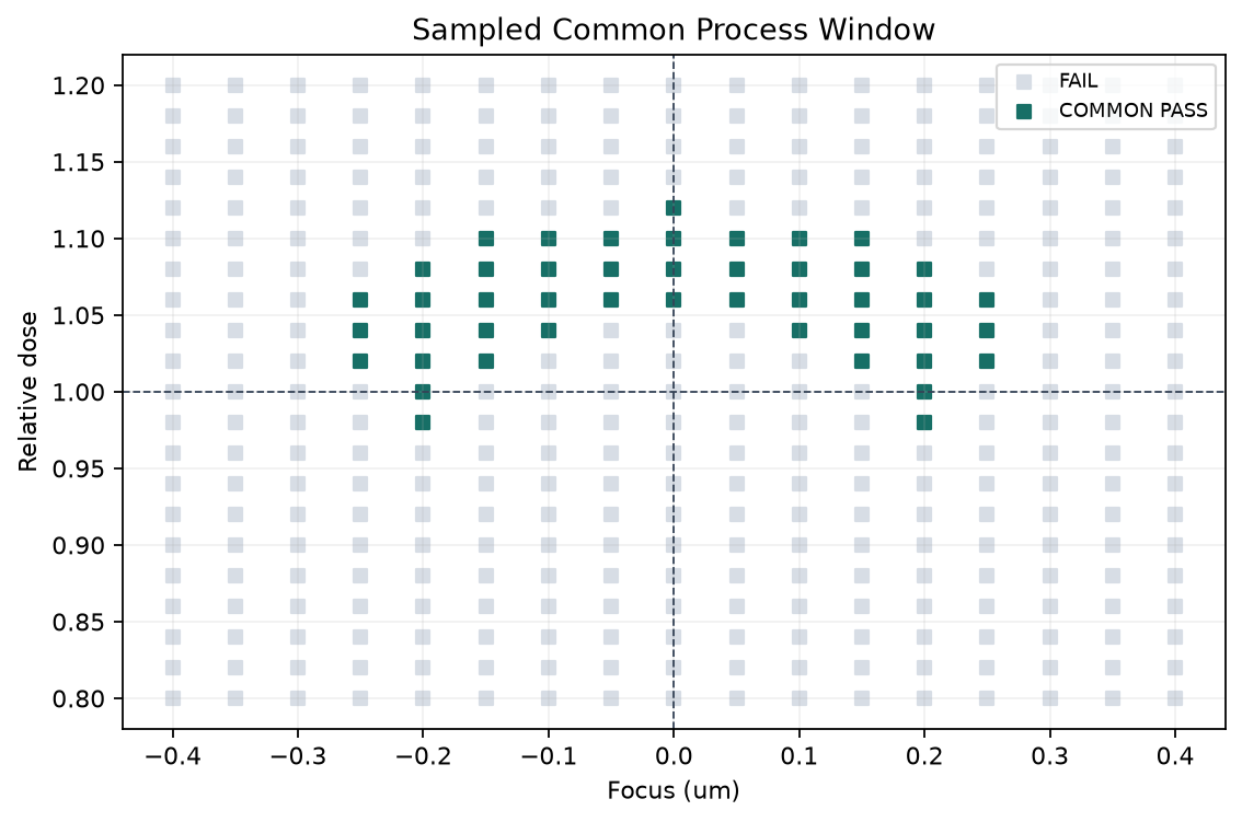
Common nominal-dose DoF is zero for both presets in this example. Matching the reference nominal CD does not ensure all candidates pass or have a wide PW. Common PW includes the three recorded locations; minimum-CD hotspot summaries exclude the reference. CD variation with focus/dose is expected; ambit comparisons must match focus/dose conditions.
Times above are single local Windows end-to-end runs with the new candidate ordering, not hosted guarantees. An earlier Render public-sample request took about 109.28 seconds with the previous candidate order; it is not a hosted benchmark of this revision. New local reference-dose CSV values match the existing reference results.
9. Interpretation and regression checks
The binary mask uses polygon transmission=1 and background=0. Contours bound the high-intensity phase I >= T_eff; they do not represent remaining positive-tone resist. A PTD opening interpretation still needs a subsequent transfer-process convention to connect it with a conductor. NTD/PTD development, etch and material stacks are not modeled. Layer names alone do not establish mask polarity or the manufacturing flow. Complementing a mask requires recomputing optics, not replacing intensity with 1-I.
- 112 unit/regression tests pass: CD/area ordering, missing-CD fallback, short-interaction retention, inverse-dose scaling, raw normalization boundaries, calibration failure, existing PW behavior, DBU/hierarchy, holes/islands, domain and export checks.
- Both new review GDS files use 0.1 nm internal DBU and preserve all 34 original physical layers with empty XOR.
- Speed detailed Region screening is off by default and nominal-only when enabled. Internal checks all three preview doses. Both export all three dose contours.
NOT_EVALUATEDand unavailable valid domains are not PASS. Marker and edge-pair counts are not independent defect counts.- One dense reference and bounded gauges do not establish full-contour EPE, convergence on every pattern, scanner/resist calibration or manufacturing signoff.
- Public documentation retains reproducible conditions, units and public-pattern coordinates, without personal paths or development dates.
10. Data downloads
Study graphs and CSV files are linked in their sections above. The following app outputs use the new ordering. Model JSON records relative dose, T_eff and reference conditions together to avoid confusing dose with threshold.
speed
- reference_dose.csv
- relative_dose_model.json
- focus_dose_measurements.csv
- contour_hotspots.json
- pya_native_combined_review.gds